In one recent project I needed to draw several maps and visualize different kinds of geographical data on it. I found the combination of R/ggplot/maps package extremely flexible and powerful, and produce nice looking map based visualizations.
Here is a short tutorial, monospace font indicates the code you need to run in R. You probably need some basic understanding of R to work through this tutorial.
- Install R. Download from http://cran.r-project.org/
- Install required R packages: maps and ggplot2.
 install.packages("maps")

install.packages("ggplot2")
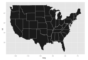
- Now import the libraries, load the US map data, and draw a map with all states.
library(ggplot2)

library(maps)

#load us map data

all_states <- map_data("state")

#plot all states with ggplot

p <- ggplot()

p <- p + geom_polygon( data=all_states, aes(x=long, y=lat, group = group),colour="white", fill="grey10" )

p
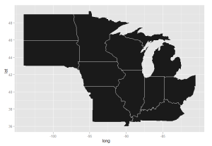
- If you only want a subset of states, subset the all_states dataframe and redraw the plot.
states <- subset(all_states, region %in% c( "illinois", "indiana", "iowa", "kentucky", "michigan", "minnesota","missouri", "north dakota", "ohio", "south dakota", "wisconsin" ) )

p <- ggplot()

p <- p + geom_polygon( data=states, aes(x=long, y=lat, group = group),colour="white", fill="grey10" )

p
- Prepare a geographical dataset, which contains the data you want to visualize onto the map. Indicate the geographical location of each data point in terms of longitude and latitude. As an example, download this file and save it as “geo.csv” into your working directory, and load it into R.
mydata <- read.csv("geo.csv", header=TRUE, row.names=1, sep=",")
- In the dataset, there are 39 universities in the midwest region, we want to visualize all these schools on the map, put a label on some of the schools, and we want to make the size of each dot proportional to the total number of enrollment in the school, and we want a legend, with the name “Total enrollment”. Sounds like a bit complicated, huh? But it’s just two lines of more code.
p <- ggplot()

p <- p + geom_polygon( data=states, aes(x=long, y=lat, group = group),colour="white" )

p <- p + geom_point( data=mydata, aes(x=long, y=lat, size = enrollment), color="coral1") + scale_size(name="Total enrollment")

 p <- p + geom_text( data=mydata, hjust=0.5, vjust=-0.5, aes(x=long, y=lat, label=label), colour="gold2", size=4 )

p
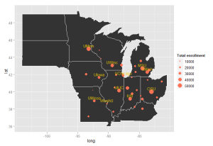
For those of you who knows R but are not familiar with ggplot, the catch is the size=enrollment option in the geom_point function. This option sets the size of the dots proportional to the number of enrollment in the dataset.
- Now we can see that there are so many schools in Chicago that they actually overlapped with each other, we want to jitter the dots a bit so we can see them better. So I changed
geom_pointfunction togeom_jitterand usedpositionoption to control the magnitude of jittering.
p <- ggplot()

p <- p + geom_polygon( data=states, aes(x=long, y=lat, group = group),colour="white" )

p <- p + geom_jitter( data=mydata, position=position_jitter(width=0.5, height=0.5), aes(x=long, y=lat, size = enrollment, color="coral1")) + scale_size(name="Total enrollment")

p <- p + geom_text( data=mydata, hjust=0.5, vjust=-0.5, aes(x=long, y=lat, label=label), colour="gold2", size=4 )

p
Some schools are jittered so much that they are in the lake now, but….. you get my point.
So what if you want to change the colors of schools to indicate some other factors, such as What state are they in?
- Use
coloroption to change the colors of the dots.
p <- ggplot()

p <- p + geom_polygon( data=states, aes(x=long, y=lat, group = group),colour="white" )

p <- p + geom_jitter( data=mydata, position=position_jitter(width=0.5, height=0.5), aes(x=long, y=lat, size = enrollment,color=state)) + scale_size(name="Total enrollment")

p <- p + geom_text( data=mydata, hjust=0.5, vjust=-0.5, aes(x=long, y=lat, label=label), colour="gold2", size=4 )

p
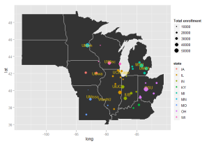
Now you can see a really colorful map… if you don’t like the colors, you can change the color scale using the scale_color_brewer function, or manually choose the color using scale_colour_manual function in ggplot.
So this is just a very simple illustration of the incredible power and flexibility of ggplot2 using maps as an example. While the grammar of ggplot2 seems a bit mysterious the first time you see it, it is actually built on the so called “grammer of graphics”. It basically allows you to build your own plot layer by layer, with absolute control of each single element in the plot.
For professional plotting, I highly recommendggplot2. http://had.co.nz/ggplot2/

